先知ppt

In a previous post, I used stock market data to show how prophet detects changepoints in a signal (). After publishing that article, I’ve received a few questions asking how well (or poorly) prophet can forecast the stock market so I wanted to provide a quick write-up to look at stock market forecasting with prophet.

在上一篇文章中，我使用股市数据来展示先知如何检测信号中的变化点（ ）。 发表该文章后，我收到了几个问题，询问先知对股票市场的预测有多好（或差），所以我想提供一个快速的文章来探讨先知对股票市场的预测。

This article highlights using prophet for forecasting the markets.  You can find a jupyter notebook with the full code used in this post .

本文重点介绍了使用先知来预测市场。 你可以找到在这篇文章中使用的完整代码jupyter笔记本电脑 。

For this article, we’ll be using . You can download this data into CSV format yourself or just grab a copy from the my github ‘examples’ directory .  let’s load our data and plot it.

对于本文，我们将使用 。 您可以下载这个数据转换成CSV格式自己或只是抓住从我的github“的例子”目录复制 。 让我们加载数据并绘制它。

market_df = pd.read_csv('../examples/SP500.csv', index_col='DATE', parse_dates=True)market_df.plot()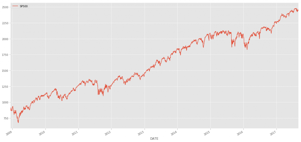

with

与

Now, let’s run this data through prophet. Take a look at  for more information on the basics of Prophet.

现在，让我们通过先知来运行这些数据。 请参阅了解有关先知基础知识的更多信息。

df = market_df.reset_index().rename(columns={'DATE':'ds', 'SP500':'y'})df['y'] = np.log(df['y'])model = Prophet()model.fit(df);future = model.make_future_dataframe(periods=365) #forecasting for 1 year from now.forecast = model.predict(future)

And, let’s take a look at our forecast.

并且，让我们看一下我们的预测。

figure=model.plot(forecast)

With the data that we have, it is hard to see how good/bad the forecast (blue line) is compared to the actual data (black dots). Let’s take a look at the last 800 data points (~2 years) of forecast vs actual without looking at the future forecast (because we are just interested in getting a visual of the error between actual vs forecast).

利用我们拥有的数据，很难看到将预测（蓝线）与实际数据（黑点）进行比较的好坏。 让我们看一下预测与实际的最后800个数据点（约2年），而不查看未来的预测（因为我们只是想了解实际与预测之间的误差）。

two_years = forecast.set_index('ds').join(market_df)two_years = two_years[['SP500', 'yhat', 'yhat_upper', 'yhat_lower' ]].dropna().tail(800)two_years['yhat']=np.exp(two_years.yhat)two_years['yhat_upper']=np.exp(two_years.yhat_upper)two_years['yhat_lower']=np.exp(two_years.yhat_lower)two_years[['SP500', 'yhat']].plot()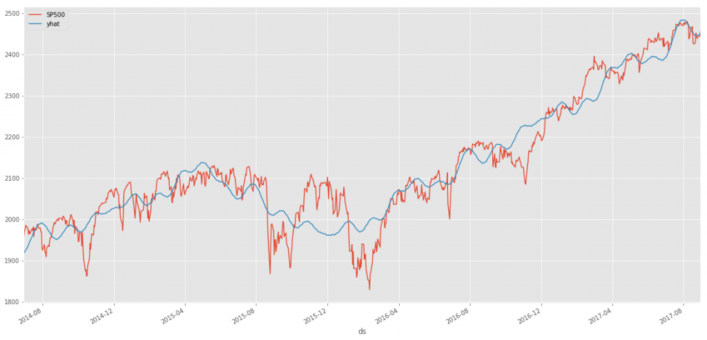

You can see from the above chart, our forecast follows the trend quite well but doesn’t seem to that great at catching the ‘volatility’ of the market. Don’t fret though…this may be a very good thing though for us if we are interested in ‘riding the trend’ rather than trying to catch peaks and dips perfectly.

从上图可以看出，我们的预测很好地遵循了趋势，但是在抓住市场的“波动性”方面似乎并不那么出色。 不过，不要烦恼……如果对我们“驾驭潮流”感兴趣，而不是试图完美地抓住高峰和低谷，这对我们来说可能是一件好事。

Let’s take a look at a few measures of accuracy.  First, we’ll look at a basic pandas dataframe describe function to see how thing slook then we’ll look at R-squared, Mean Squared Error (MSE) and Mean Absolute Error (MAE).

让我们看一些准确性的度量。 首先，我们来看一个基本的熊猫数据框 describe 函数来查看事物的外观，然后我们将查看R平方，均方误差（MSE）和平均绝对误差（MAE）。

two_years_AE = (two_years.yhat - two_years.SP500)print two_years_AE.describe()count    800.000000mean      -0.540173std       47.568987min     -141.26577425%      -29.38354950%       -1.54871675%       25.878416max      168.898459dtype: float64

Those really aren’t bad numbers but they don’t really tell all of the story. Let’s take a look at a few more measures of accuracy.

这些确实不是一个坏数字，但是他们并没有真正讲述所有的故事。 让我们看一下更多的准确性度量。

Now, let’s look at R-squared using sklearn’sr2_score function:

现在，让我们使用sklearn的R平方 r2_score 功能：

r2_score(two_years.SP500, two_years.yhat)

We get a value of 0.91, which isn’t bad at all. I’ll take a 0.9 value in any first-go-round modeling approach.

我们得到0.91的值，这还不错。 在任何首轮建模方法中，我都会采用0.9的值。

Now, let’s look at mean squared error using sklearn’smean_squared_error function:

现在，让我们看一下使用sklearn的均方误差 mean_squared_error 功能：

mean_squared_error(two_years.SP500, two_years.yhat)

We get a value of 2260.27.

我们得到的值为2260.27。

And there we have it…the real pointer to this modeling technique being a bit wonky.

到了这里，指向该建模技术的真正指针有些古怪。

An MSE of 2260.28 for a model that is trying to predict the S&P500 with values between 1900 and 2500 isn’t that good (remember…for MSE, closer to zero is better) if you are trying to predict exact changes and movements up/down.

如果您要预测准确的变化和向上/向下运动，则试图预测1900-2500之间的S＆P500的模型的MSE为2260.28并不是很好（记住...对于MSE，接近零更好） 。

Now, let’s look at the mean absolute error (MAE) using sklearn’s mean_absolute_error function. The MAE is the measurement of absolute error between two continuous variables and can give us a much better look at error rates than the standard mean.

现在，让我们看一下使用sklearn的平均绝对误差（MAE） mean_absolute_error 功能。 MAE是两个连续变量之间的绝对误差的度量，可以使我们对误差率的了解比标准均值好得多。

mean_absolute_error(two_years.SP500, two_years.yhat)

For the MAE, we get 36.18

对于MAE，我们得到36.18

The MAE is continuing to tell us that the forecast by prophet isn’t ideal to use this forecast in trading.

MAE继续告诉我们，先知的预测在交易中使用此预测并不理想。

Another way to look at the usefulness of this forecast is to plot the upper and lower confidence bands of the forecast against the actuals. You can do that by plotting yhat_upper and yhat_lower.

检验此预测有用性的另一种方法是相对于实际绘制预测的上下置信带。 您可以通过绘制yhat_upper和yhat_lower来实现。

fig, ax1 = plt.subplots()ax1.plot(two_years.SP500)ax1.plot(two_years.yhat)ax1.plot(two_years.yhat_upper, color='black',  linestyle=':', alpha=0.5)ax1.plot(two_years.yhat_lower, color='black',  linestyle=':', alpha=0.5)ax1.set_title('Actual S&P 500 (Orange) vs S&P 500 Forecasted Upper & Lower Confidence (Black)')ax1.set_ylabel('Price')ax1.set_xlabel('Date')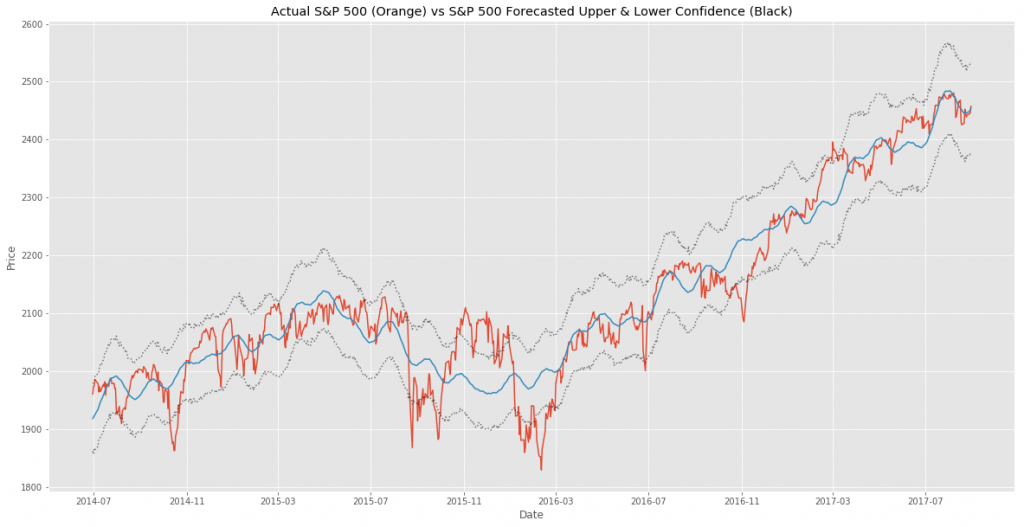

In the above chart, we can see the forecast (in blue) vs the actuals (in orange) with the upper and lower confidence bands in gray.

在上面的图表中，我们可以看到预测（蓝色）相对于实际（橙色），上下置信带为灰色。

You can’t really tell anything quantifiable from this chart, but you can make a judgement on the value of the forecast. If you are trying to trade short-term (1 day to a few weeks) this forecast is almost useless but if you are investing with a timeframe of months to years, this forecast might provide some value to better understand the trend of the market and the forecasted trend.

您实际上无法从此图表中得出任何可量化的信息，但是可以对预测值进行判断。 如果您尝试进行短期交易（1天到几周），则该预测几乎没有用，但是如果您的投资期限为数月至数年，则此预测可能会提供一些价值，以更好地了解市场趋势并预测趋势。

Let’s go back and look at the actual forecast to see if it might tell us anything different than the forecast vs the actual data.

让我们回过头来看看实际的预测，看它是否可以告诉我们与预测和实际数据不同的地方。

full_df = forecast.set_index('ds').join(market_df)full_df['yhat']=np.exp(full_df['yhat'])fig, ax1 = plt.subplots()ax1.plot(full_df.SP500)ax1.plot(full_df.yhat, color='black', linestyle=':')ax1.fill_between(full_df.index, np.exp(full_df['yhat_upper']), np.exp(full_df['yhat_lower']), alpha=0.5, color='darkgray')ax1.set_title('Actual S&P 500 (Orange) vs S&P 500 Forecasted (Black) with Confidence Bands')ax1.set_ylabel('Price')ax1.set_xlabel('Date')L=ax1.legend() #get the legendL.get_texts()[0].set_text('S&P 500 Actual') #change the legend text for 1st plotL.get_texts()[1].set_text('S&P 5600 Forecasted') #change the legend text for 2nd plot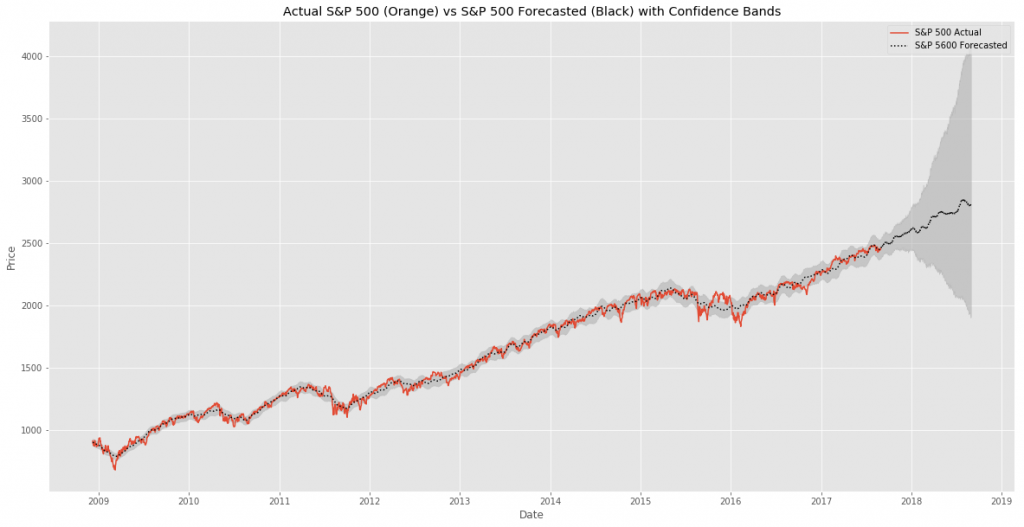

This chart is a bit easier to understand vs the default prophet chart (in my opinion at least). We can see throughout the history of the actuals vs forecast, that prophet does an OK job forecasting but has trouble with the areas when the market become very volatile.

与默认的先知图表相比，此图表更易于理解（至少在我看来）。 我们可以看到，在实际值与预测值的历史记录中，先知可以很好地进行预测，但是当市场变得非常动荡时，该地区存在问题。

Looking specifically at the future forecast, prophet is telling us that the market is going to continue rising and should be around 2750 at the end of the forecast period, with confidence bands stretching from 2000-ish to 4000-ish.  If you show this forecast to any serious trader / investor, they’d quickly shrug it off as a terrible forecast. Anything that has a 2000 point confidence interval is worthless in the short- and long-term investing world.

先知特别看一下未来的预测，他告诉我们市场将继续上涨，在预测期结束时，价格应在2750左右，信心区间将从2000欧元扩展到4000欧元。 如果您将此预测显示给任何认真的交易者/投资者，他们都会Swift将其视为可怕的预测。 在短期和长期投资世界中，任何具有2000点置信区间的东西都是毫无价值的。

That said, is there some value in prophet’s forecasting for the markets? Maybe. Perhaps a forecast looking only as a few days/weeks into the future would be much better than one that looks a year into the future.  Maybe we can use the forecast on weekly or monthly data with better accuracy. Or…maybe we can use the forecast combined with other forecasts to make a better forecast. I may dig into that a bit more at some point in the future. Stay tuned.

也就是说，先知对市场的预测是否有价值？ 也许。 也许只预测未来几天/几周的预测要比预测未来一年的预测好得多。 也许我们可以将预测用于每周或每月的数据中，从而获得更好的准确性。 或者……也许我们可以结合使用其他预测来做出更好的预测。 我可能会在将来的某个时候对它进行更多的研究。 敬请关注。

翻译自:

先知ppt